COMPACT -
Comparative Package for Clustering Assessment (Version 2.0)
By
Roy Varshavsky, Michal Linial,
Outline
COMPACT is a
COMPACT is a five-step wizard that envelops some basic Matlab clustering methods and introduces the Quantum clustering algorithm that was originally proposed by Prof. David Horn and Assaf Gottlieb (see The Method of Quantum Clustering, for more details). COMPACT provides a flexible and customizable interface for clustering data with high dimensionality.
COMPACT allows both textual and graphical display for the clustering results.
How to install
COMPACT is a self-extracting package. In
order to install and run the COMPACT
tool,
follow these three
easy steps:
1.
Download the COMPACT.zip packaged to your local
drive.
2.
Add the COMPACT destination directory to your
Matlab path.
3.
Within Matlab, type 'compact' at
the command prompt.
Steps
In order to run the COMPACT properly, you should follow five steps. These steps are mandatory and cannot be skipped. However, in each one of the steps you can return to the previous step(s) and change your settings.
1.
Input
parameters
COMPACT receives two input parameters, which are Matlab base workspace variables (i.e., must be defined in Matlab workspace before running the COMPACT).
À
Data (Mandatory field) - two-dimensional matrix
of doubles. Represents the elements (objects to be clustered can be either
columns or rows).
À
Real classification (Optional field) - one-dimensional
vector. Represents the real classification of the elements (i.e., the class of
the i-th element appears in the i-th place in the vector).
Therefore, the vectorÆs length must be equal to the number of elements in the
Data matrix (an error occurs otherwise).
The two input parameters can be either typed
in or selected from the base workspace.
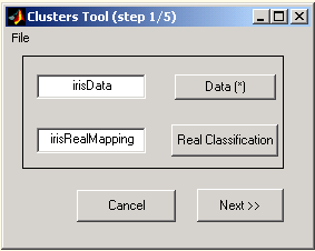
Figure 1: Input parameters
a. Selecting variables from base
workspace
Press the 'Data' or the 'Real Classification' button and double click the required variable from the list in the 'Select Variable' dialog.
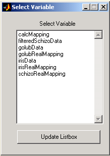
Figure 2: Variables selection dialog
As explained above, the 'Real classification' parameter is optional. If this field remains empty, a popup question appears.
b. Skipping Real Classification input
If you leave the real classification empty, you will be prompted and asked whether to leave the real mapping empty (press 'Yes' button) or specify this input ('No' button). In case where real classification isn't defined, graphical displays and clustering evaluations will be modified and limited (see steps 4 and 6, respectively).
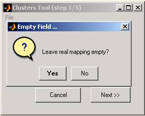
Figure 3: Missing real classification field
2.
Determining the matrix
shape and vectors to cluster
COMPACT reads the Data matrix and displays its schematic shape. You will be asked to select the entities to cluster: rows or columns. When rows are selected, each entity is a row with n(columns) dimensions (and vice versa).
For your convenience, a flip option is available. If you choose to flip the matrix, the schematic display will change accordingly and the Data matrix will be transposed.
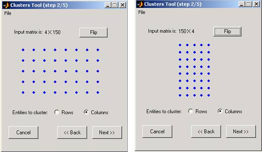
Figure 4: Matrix shape determination
3.
Preprocessing
Procedures
The preprocessing window consists of two sections:
a. Components' variance graphs û the relative and accumulated variances of the principal components as processed by the SVD (singular values)
method,
are plotted. The variance of component i (Vi)
is defined as:
 .
.
b. Preprocessing parameters -
º Use SVD method - yes/no check box.
º Normalized selected vectors - yes/no check box (available only when SVD option is selected).
º Relevant dimensions - you can select either the first x dimensions (first field), a range of dimensions (second field: from dimension #i to dimension #j) or a selection of dimensions (e.g., 1, 3-5, 7).
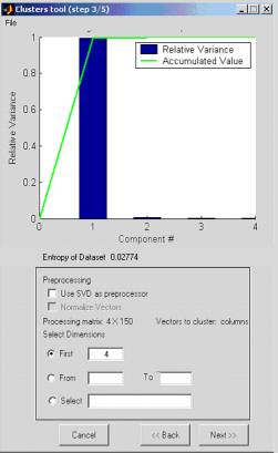
Figure 5: Preprocessing procedures
4.
Points distribution preview and
clustering method selection
The elements of the Data matrix are plotted (3D plot of the first 3 selected dimensions or 2D plot when only 2 dimensions are chosen). Each original class is displayed in a different color. The original classification is taken from the 'Real classification' input parameter (see step 1). If no 'Real classification' is available, all points are plotted in black.
At this stage you are asked to select the clustering method: k-means, fuzzy c-means, competitive neural network or QC (Quantum Clustering algorithm).
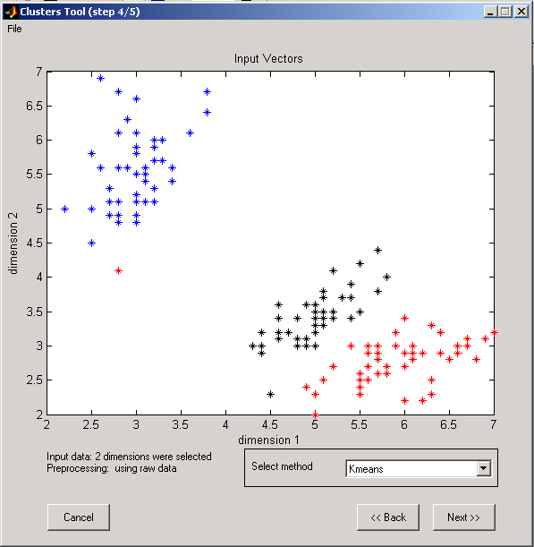
Figure 6: Clustering method determination
5.
Parameters for clustering
algorithms
a. Parameter for K-means algorithm (Matlab kmeans function) - number of clusters
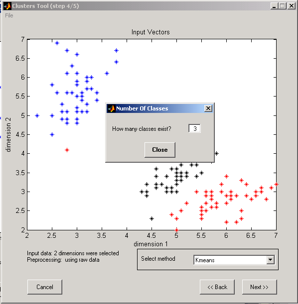
Figure 7: K-means input parameter
b. Parameters for Fuzzy C-means algorithm (Matlab fcm function):
º Exponent for the partition matrix U (default: 2.0)
º Maximum number of iterations (default: 100)
º Minimum amount of improvement (default: 1e-5)
º Info display during iteration (default: Yes).
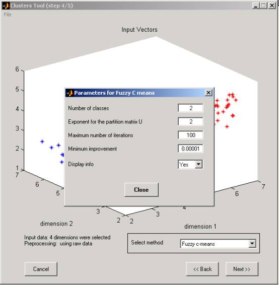
Figure 8: Fuzzy C-means input parameters
c. Parameters for Competitive neural network algorithm:
º Learning rate (0 - 1)
º Number of clusters
º Number of learning iterations.
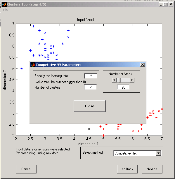
Figure 9: Competitive Network Input parameters
d. Parameters for Quantum Clustering algorithm*
º Sigma value
º Number of steps
* For more details see The Method of Quantum Clustering.
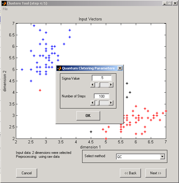
Figure 10: Quantum clustering Input parameters
6.
COMPACT results
Once the COMPACT finishes its run, the results are displayed in both graphical and textual formats.
a.
Real classification plot (upper left graph): same as
in step 4
b. AlgorithmÆs classification (upper right graph):
points are plotted by the same rule as in the Real Classification graph, but are
tagged by the algorithm (k-means, Competitive net or QC).
c.
Classification alternative display (lower right
graph): Assuming that the points are ordered by the real classification (i.e.,
the Real Classification array looks like: 1 1...2 2...3 3...), each change in the
background (white-gray-white...) represents a new cluster in the Real
classification. Each one of the points is represented as a bin whose location on
the x-axis equals its location in the Real classification and in the Data
matrices, and its location on the y-axis represents the tag proposed by the
algorithm. Perfect classification is therefore represented as homogenous
rectangles.
d. Purity, Efficiency and Jaccard scores (lower left
graph): These criteria for clustering assessment and are defined as
follows:
![]()
where:
º n11 is the number of pairs that are classified together, both in the real classification and in the algorithm's classification.
º
n10 is the number of pairs that are
classified together in the real classification, but not in the algorithm's
classification.
º
n01 is the number of pairs that are
classified together in the algorithm's classification, but not in the real
classification.
e.
Textual summary of the clustering results (lower
right textual area).
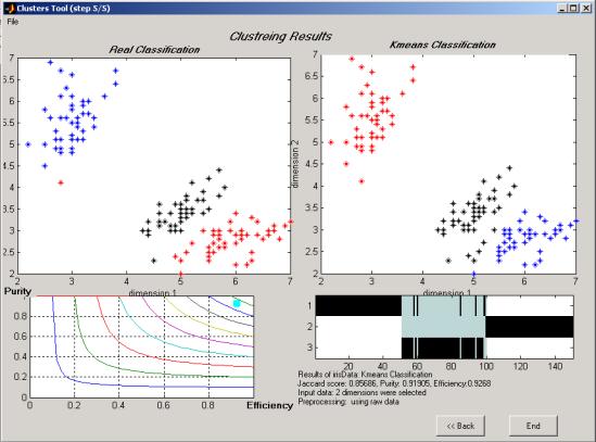
Figure 11: COMPACT results and clustering scores
f.
Starting from version 1.3, the results can be displayed
also in a log window: the Clusters Results Log dialog is a window that
displays the summary of the clustering results and quality in a textual way (see
Figure 12). The log
window is invoked by pressing the æView LogÆ button from the COMPACT result step.
This summary can be saved as a text (.txt) or matlab (.mat) files (menu:
File/Save/à)
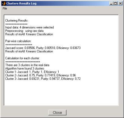
Figure 12: COMPACT textual results
7.
COMPACT output
Pressing the 'End' button at this stage will terminate the application. A new variable is then added to the Matlab workspace: calcMapping.
The calcMapping variable is a one-dimensional vector that represents the calculated classification of the elements (i.e., the proposed class of the i-th element appears in the i-th place in the vector). Actually it has similar properties to the RealClassification input parameter.
8.
Optional extensions
COMPACT is a set of self
explanatory and documented Matlab functions and as such can be extended. Users
that are familiar with Matlab and wish to change features in the current tool
are welcome to do so. In addition, we designed this tool that adding a new
clustering method is done by changing only one function (see COMPACT
extension).
9. Requirements
-
Project name: COMPACT - Comparative Package for Clustering Assessment
-
Project home page: http://adios.tau.ac.il/compact, http://www.protonet.cs.huji.ac.il/compact (alternative)
-
Operating system(s): Platform independent tested on MS-Windows (2000, XP), Linux and Unix
-
Programming language: Matlab
-
Other requirements: Matlab 7 or higher (toolboxes: fuzzy logic toolbox, version 2.1, Neural Network Toolbox 4.0.1, statistics toolbox, version 4.1).
-
License: Matlab
-
Any restrictions to use by non-academics: currently open for all academic users. Adequate referencing required. Non-academic users are required to apply for permission to use this product.
Example
iris.mat is a
workspace that includes two variables: (a) irisData: a 4X150 double array and
(b) irisRealClassification: a 1X150 real mapping array.